Electrogravitics - A Crash Course, Part 1.
The atom as field generator,
 
1.1
Introduction:
In order to understand gravity as an electro-magnetic phenomena, we must first separate the primary cause and effect form the secondary and tertiary effects.  Included in these secondary and tertiary effects are curved space, red shift, and time dilation.  Implicit in the term "Electrogravitics" is the assumption that electro-magnetism is the root cause of the gravitational effect.  This assumption is not new.  Both James C. Maxwell and Michael Faraday believed in the electro-magnetic basis of gravitational interactions, though neither was able to marshal the needed experimental evidence or mathematical models to prove their assertion.  Many key pieces of supporting evidence and physical models required to understand the nature of gravity did not exist until the beginning of the 20th century.

 
1.2
Primary cause and effect:
The fundamental questions we must answer are…
1. What is the nature and source of the field that matter generates we commonly call gravity?
2. What is the nature and seat of interaction between this field and matter that causes an attractive force to arise?
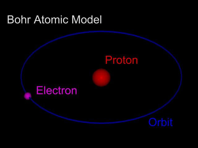
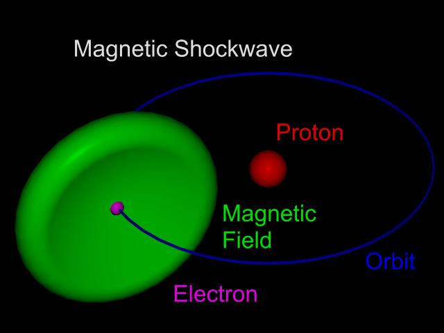
 
1.2.1
The Atom as a gravitational field generator:
For the sake of clarity, we shall limit this discussion to hydrogen in a non-ionized state and shall use the Bohr atomic model of the atom (figure 1).  The concepts discussed herein may be generalized to include more complex atoms, atoms based on newer more subtle models and ionized or plasma based systems such as stars.  In the Bohr model of hydrogen we have one electron in orbit around a single proton.  The electric field binds the electron to the proton hence the atom appears to be electrically neutral from a distance. The electron continues to orbit because there is no mechanism by which it can dissipate the orbital energy.  This is a natural form of superconductivity.

 
Figure 1

 
1.2.2
First approximations:
On first approximation, the electron can be thought of as a "current loop" centered around the proton. This current loop will have a magnetic field associated with it.  The geometry of the magnetic field is defined by the Left Hand Rule (it's negatively charged).  If we grab the loop with our left hand such that our thumb points in the direction of electron rotation, our fingers curl in the direction of the magnetic field.  Therefore to first approximation the magnetic field associated with the orbital electron can be viewed as a torus centered on the orbital path of the electron.  Unlike the electric field lines which are confined to the vicinity of the atom, the magnetic field is NOT restricted to the atom's immediate surroundings.  This field structure reaches quite literally to the stars, attenuated of course by the inverse square rule. Note that most matter appears non-magnetic because it is composed of many non-aligned atoms and overall the individual magnetic field vectors sum to zero.

 
1.2.3
Second approximations:
The current loop model has an obvious flaw.  The electron is a particle and therefore discontinuous in nature.  The electron exists at one point in it's orbit at any given instant.  This means the electron's magnetic field must also be discontinuous in nature.  In other words there is a magnetic impulse or shock wave connected to, and traveling coincident with the electron as it circulates around it's orbit (figure 2).  A thought experiment is helpful at this point.  What would this magnetic field look like to an observer located in the orbital plane and an arbitrary distance (say 100,000 orbital diameters) away from the atom?  Assuming the observer is oriented so the orbital plane is horizontal, he/she would "see" a magnetic shock wave with a velocity vector in the horizontal plane and the magnetic field vector in the vertical plane.  In other words the two vectors (velocity & magnetic) would be at right angles to each other.  This is VERY important and needs generalizing.  No mater how we orient the observer with respect to the atom, the velocity vector and magnetic field vector will remain at right angles to each other.  Study the geometry until you have satisfied your self the above statement is true in all cases.  A second and more subtle observation also comes to light from this thought experiment.  In any orientation where the velocity vector is reversed so is the magnetic vector.  At first glance this may seem trivial but as we shall see, it has profound consequences...
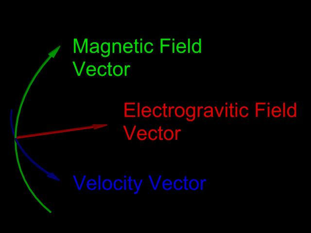
 
Figure 2

 
1.3.1
Moving magnetic fields:
Basic electro-magnetic theory teaches that a moving magnetic field creates an electric field vector or EMF (electro-motive force) that is at right angles to both the velocity vector and the magnetic field vector. The magnitude and sign of the electric field vector is the product of the velocity and magnetic field magnitudes and signs.  Mathematicians call this a Cross Product and use an "X" to indicate the operation.  If B is our magnetic vector and V is our velocity vector, then E our electric vector is equal to B X V.  H. A. Lorentz first formulated this relationship in the late 1890's as part of the Lorentz Force Equation: F = qE + q(B X V).

 
1.3.2
The electrogravitic field vector:
In 1.2.3 we found that atoms generate a B X V field structure.  In 1.3.1 we found that an electric field arises at right angles to both B and V.  Returning to our thought experiment in 1.2.3 we see the induced electric field vector points along an axis connecting the observer to the generating atom (figure 3).  This is true regardless of how we orient the atom or the observer.  This symmetry is responsible for the body central nature of the gravitational field vector.

 
Figure 3

 
1.3.3
The electrogravitic field sign:
As we noted in 1.2.3 any orientation that reversed the velocity vector, also reversed the magnetic field vector as well.  We then found in 1.3.2 the magnitude and sign of the electric field vector was equal the a cross product "X" term (B X V).  These last two statements when coupled together, produce an electric vector that is unidirectional regardless of the spin direction or orientation of the generating atom with respect to the observer.  In summary, even though the magnetic fields of any large collection of atoms cancel (except when spin aligned), their B X V components will constructively sum because two negative values, when multiplied (product term), always yield a positive result.  This asymmetry is the underlying reason we do not observe gravitational repulsion in nature.  Profound indeed!

 
1.3.4
The electrogravitic field magnitude:
As we travel away from the generating atom (in the orbital plane), the magnetic field magnitude attenuates as the inverse square of distance.  However the velocity magnitude rises proportionally with distance.  In other words as we double the distance the magnetic field magnitude drops to 1/4 of it's original value while the velocity magnitude doubles.  Therefore the B X V product magnitude falls at a rate proportional to the distance from the generating atom (1/r).  At first glance this may seem paradoxical.  Isn't the gravitational force inverse square?  As we shall see in part 2, a 1/r magnitude is exactly what is required to generate an inverse square force as the overall gravitational interaction...


End
Electrogravitics - A Crash Course Part 1