2.1.1

Atomic response to a uniform electric field:

All atoms contain equal quantities of both positive and negative electric charge and are therefore, electrically neutral.  The response of an atom to an external electric field depends on field geometry.  In a uniform electric field, the atom is not deflected.  The force on the proton is canceled by an equal and opposite force on the electron.  These equal and opposite forces do create internal stress.  In other words the electron orbit is deformed since part of the atomic binding energy is being diverted into opposing the externally applied electric field.

2.1.2

Atomic response to a non-uniform electric field:

In a non-uniform electric field, the atom is deflected because the force on the proton and electron while opposite, are no longer equal to each other.  What is surprising is the nature of the deflection.  The atom is always deflected to the vicinity of highest electric field density regardless of field polarity.  This result is due to deformation of the electron orbit.  Upon reflection it is obvious that orbital deformation will always result in the attracted part of the atom being on average in a stronger electric field than the repulsed part of the atom (figure 4).  Therefore the force exerted on the attractive part of the atom will always be greater (on average) than the force exerted on the repulsive part and deflection will be in the direction of attraction regardless of electric field polarity.

2.1.3

Strong field limit:

The discussion in 2.1.1 & 2.1.2 assumes the external electric field strength is small compared to the electric binding force that holds the electron in orbit.  Under these conditions orbital deformation is very close to a linear function of external electric field.  As the external electric field strength approaches the orbital binding energy, the degree of orbital deformation becomes increasingly non-linear.  When the external electric field is equal to the orbital binding energy the electron orbit becomes unstable and extremely non-linear.  This is the strong field limit.  Any further increase in external field results in orbital disruption and ionization.  Please note that non-linearity in orbital deformation exists at all electric field strengths but does not become pronounced unless we approach the strong field limit.

2.1.4

Electric field shielding:

The field that exists between two conductors of differing electric potential can be screened or shielded in a given space by enclosing that space with a conductive material.  Michael Faraday was the first person to note this effect and the shield is commonly called a faraday shield or cage.  An electric field created by a moving magnetic field (B X V) cannot be shielded in this manner.  Modern transformers take advantage of this by introducing a faraday shield between the primary and secondary windings.  Electrical noise in the primary winding is shielded from the secondary winding while magnetic induction between the windings is unaffected.  In atoms with multiple electron shells a similar condition prevails.  The electrons in the inner shells are faraday shielded by the outer electron shells, however a magnetically induced electric field (B X V) is in no way impeded or attenuated by the outer electron shell shielding.

2.1.5

The atom as an electrogravitic receiver:

To recap part 1. (a) The electrogravitic field is an induced electric field caused by a moving magnetic field (1.3.1).  (b) The electric field vector always exists on an axis connecting the generating atom with the observation point (1.3.2).  (c) The field strength is inversely proportional to the distance separating the generating atom and observer [1/r] (1.3.4).  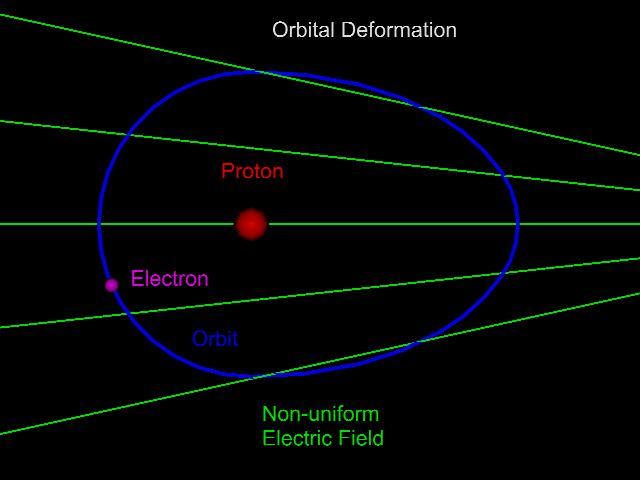Now lets place our "test atom" 100,000 orbital diameters away from a "generating atom" (part 1) and see what happens.  First, because the electrogravitic field is non-linear [1/r], the test atom is deflected in the direction of higher field strength (2.1.2) I.E. along the radial axis connecting the generator and the test atom.  Second, electron orbital deformation in the test atom is proportional to the electrogravitic field strength (2.1.2) and since the force on the test atom is the net difference between attractive and repulsive components.  Halving the distance between the test atom and the generator atom, doubles the electrogravitic field strength thereby doubling orbital deformation and quadrupling the attractive force.  Consequently the electrogravitic force on the test atom is inverse square [1/r²] even though the electrogravitic field is just inverse [1/r].

2.1.6

The real world:

For the sake of clarity we have considered the generating atom to be the cause of the electrogravitic field, and the test atom to be the receiver of and affected by the electrogravitic field.  In the real universe, both atoms are simultaneous generators and receivers.  Therefore the electrogravitic force is proportional to the product term of the interacting masses.

2.1.7

Summary:

We have now defined the basic cause of, and the effect on matter by the electrogravitic field.  We have answered the questions posed in 1.1.  Further, as required by classical physics, our electrogravitic force is inverse square with distance (2.1.5), body centered in vector (1.3.2 & 2.1.1), proportional to the product term of the masses (2.1.6), always atractive (1.3.3 & 2.1.2), and can not be shielded by conventional methods (2.1.4).  In part 3 of electrogravitics - a crash course, we shall examine some practical engineering examples.

End

Electrogravitics - A Crash Course Part 2